Loading the frozen snapshot…
Week 2 · Models & null models
One hero gone. Who loses their way?
Imagine Wikipedia as a transport map: articles are stations, and links are routes between them. If one station closes, can the others still reach each other? Follow a journey and find out.
Closing a station removes an article and its links from our model; it does not change Wikipedia.
Will your journey survive?
Of the 303 articles, 277 form one connected group: each can reach every other through links. We test removals inside this group, following links in either direction. “Cut off” means losing the route to the largest group left after a removal. Pick a journey below, then close a station to see what changes.
Marvel Transit · journey ticket
Choose your journey
Normal service
After closure
Loading the route…
A route view, not the full network. Each stop is a Wikipedia article; positions only show the order of the journey. Journey predictions are not scored or saved.
Predict the total disruption instead
Compared with chance
Is this more disruption than the link counts explain?
We rearranged the core’s links 1,000 times, keeping every article’s number of neighbours and each starting network connected. Then we removed the same article.
This tests a specific rewiring model. It is not the chance of a real-world failure or proof of why these links exist.
Inspect the shuffle distribution and methods
The comparison that matters
Same degrees. Different wiring.
The benchmark rewires the 277-station core while preserving each station’s degree. Each starting network must be connected. Then the same station is removed.
The 1,000 recorded draws are a degree-controlled benchmark, not a probability of real-world failure. “Stranded” means outside the largest remaining component.
What we found
A busy station is not always a vital connection.
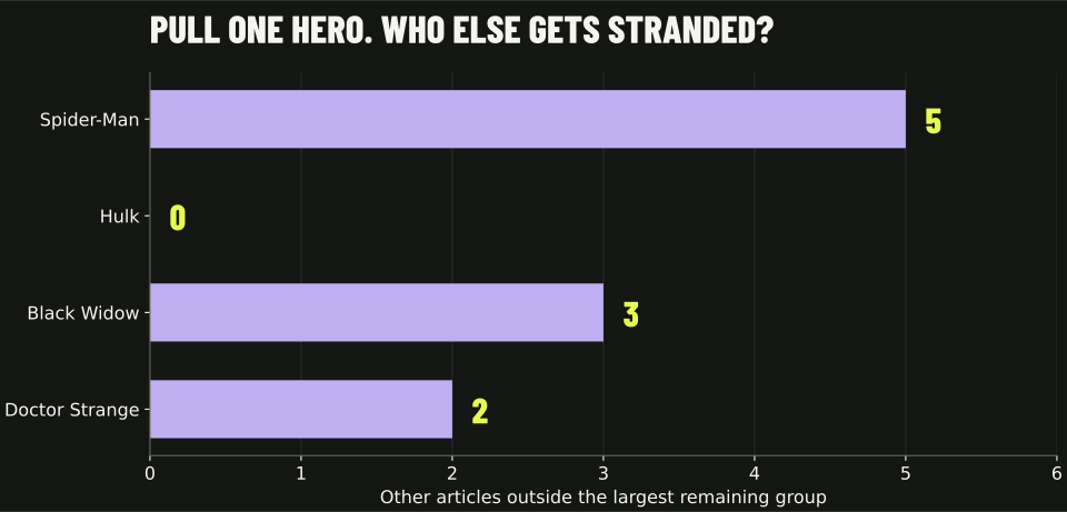
In the connected group of 277 Wikipedia articles, removing Spider-Man and its links cuts five other articles off from the largest group left. Removing Hulk cuts off none—even though Hulk has 65 neighbours. What matters is whether other routes remain, not just how many links a station has.
We also made 1,000 alternative maps. Each article kept the same number of neighbours, but we changed who connected to whom. Only nine of those maps lost at least five articles when Spider-Man was removed. Its particular connections matter.
What surprised us
Black Widow has 25 links, far fewer than Hulk's 65, yet removing Black Widow strands 3 articles while removing Hulk strands none. Link count alone does not predict which station is a bridge.
THE TAKEAWAY
Count the alternative routes, not just the connections.
A station with many neighbours can still be easy to bypass. A less busy one can be the only way through. Comparing with rearranged maps helps us ask whether the pattern depends on the specific connections.
Curious? Go deeper.
Charts, data and methods for anyone who wants to check the details.
Missing two more models? Play Screen Test.
This post covers the A null model that rewires the links at random while every node keeps its exact number of links., the A network in which every link joins a pair of nodes picked uniformly at random. G(n, m) is the version with a fixed number of links., the On average your friends have more friends than you do, because people with many friends appear in many friend lists. and How often two neighbours of a node are also linked to each other, closing a triangle., and compares The number of links on the shortest route between two nodes. against both nulls. Screen Test adds two more candidates, A model that starts from a ring where each node links to its nearest neighbours and rewires a few links at random, giving many triangles and short paths. and A model that grows a network one node at a time, each newcomer linking preferentially to nodes that already have many links, which makes hubs., and the The high end of the spread of link counts: how many nodes have very many links.: three mechanisms audition against the Marvel network, and only one measurement says which properties survive.
Play Screen Test ↗Explore the explanations & evidence
Another example: do linked articles form clusters?
When two articles both link to a third, do they also link to each other? Clustering measures how often these small triangles close. We compare the observed network with two ways of rearranging its links.
Clustering stays high after we hold degrees fixed. Its size alone is not the finding; its excess over a suitable baseline is.
Means from 1,000 draws per null. This full-network comparison is separate from the connected-core removal test above.
Inspect the full comparison →Could the result happen by chance?
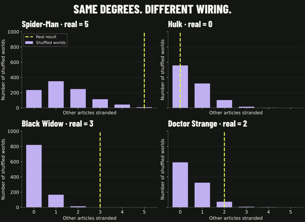
As a shuffle test: Spider-Man strands 5 against a shuffle mean of 1.41, empirical \htmlClass{x-p-empirical}{p} = 0.010; Black Widow strands 3 against 0.19, \htmlClass{x-p-empirical}{p} = 0.001 — no rewired world managed more than 2. Doctor Strange’s 2 against 0.51 gives \htmlClass{x-p-empirical}{p} = 0.086, and Hulk’s 0 against 0.58 is the most ordinary outcome there is (\htmlClass{x-p-empirical}{p} = 1.0).
Black Widow was chosen after scanning all 277 removals, so her The chance of a result at least this extreme if only the null model's randomness were at work. describes her rank rather than testing a prior guess. The four p-values are Counting only null results as extreme as the real one in the same direction. and Not corrected for testing several results at once, so one small p among many can still be luck..
A z-score describes distance from the null mean in standard deviations; it does not require a normal distribution. These small, skewed counts are easier to interpret through their histograms and empirical tail probabilities. Normal-tail significance should not be inferred from their z-scores.
What else changes when we rearrange the links?
Twelve measurements against two null models
12 QUANTITIES · 2 NULLS · 1,000 DRAWS EACHA null model supplies a baseline. We compare the observed network with networks that preserve selected properties and randomize the rest.
We measured twelve quantities on the full 303-article snapshot and on 1,000 draws from each of two null models.
Null A · the degree-preserving shuffle
Take the real network and rewire A–B and C–D into A–D and C–B, 28,680 times over. Every article keeps its exact degree; who links to whom is scrambled. Spider-Man still has 106 links and the 17 isolates still have none — degree zero cannot gain a link this way.
Keeps the node count, edge count and every degree; randomizes the wiring subject to those constraints.
Null B · random G(n, m)
Throw the wiring away entirely: 303 nodes, 1,434 links, every link between a uniformly random pair. Degrees are redrawn by chance, so the hubs vanish and so do the isolates — with an average degree of 9.5, chance almost never leaves an article unlinked.
Keeps: \htmlClass{x-n-nodes}{n} and \htmlClass{x-m-links}{m}. Destroys: the degree sequence too.
The whole table
| Quantity | Real | Shuffle | z | p | G(n, m) | z |
|---|---|---|---|---|---|---|
| Average clustering C | 0.307 | 0.143 | +19.8 | 0.001 | 0.032 | +93.9 |
| Transitivity | 0.182 | 0.115 | +15.6 | 0.001 | 0.031 | +58.4 |
| Triangles | 1,839 | 1,158 | +15.6 | 0.001 | 142 | +142.8 |
| Islands (connected components) | 19 | 18.04 | +5.0 | 0.039 | 1.02 | +131.6 |
| Largest component | 277 | 285.9 | −23.3 | 0.001 | 303.0 | −190.2 |
| Average distance in the largest component | 2.674 | 2.631 | +2.9 | 0.005 | 2.778 | −24.0 |
| Degree assortativity | −0.098 | −0.120 | +2.0 | 0.024 | −0.008 | −3.5 |
| Mean degree at the end of a random link | 22.08 | 22.08 | — | — | 10.43 | +152.3 |
| Mean degree of a random character’s random friend | 24.22 | 24.19 | +0.1 | 0.469 | 10.44 | +168.5 |
| Chance your random friend is at least as linked | 0.753 | 0.763 | −3.5 | 0.001 | 0.635 | +30.7 |
| Characters no friend out-links | 2 | 1.26 | +1.3 | 0.205 | 16.68 | −5.1 |
| Biggest hub’s share of all link ends | 3.70% | 3.70% | — | — | 0.67% | +57.7 |
Two rows have no z and no p. The mean degree at the end of a random link is \htmlClass{x-edge-degree}{\htmlClass{x-k2-avg}{\langle k^2 \rangle} / \htmlClass{x-k-avg}{\langle k \rangle}}, and the hub’s share is \htmlClass{x-hub-links}{106} / \htmlClass{x-link-ends}{2{,}868}: both are functions of the degree sequence alone, so the degree-preserving shuffle reproduces them to every decimal place across all 1,000 draws. The standard deviation is exactly zero and a z-score would be a division by it. That is not a broken measurement — it is the null telling you the quantity carries no information beyond the degrees.
What changes under the shuffle
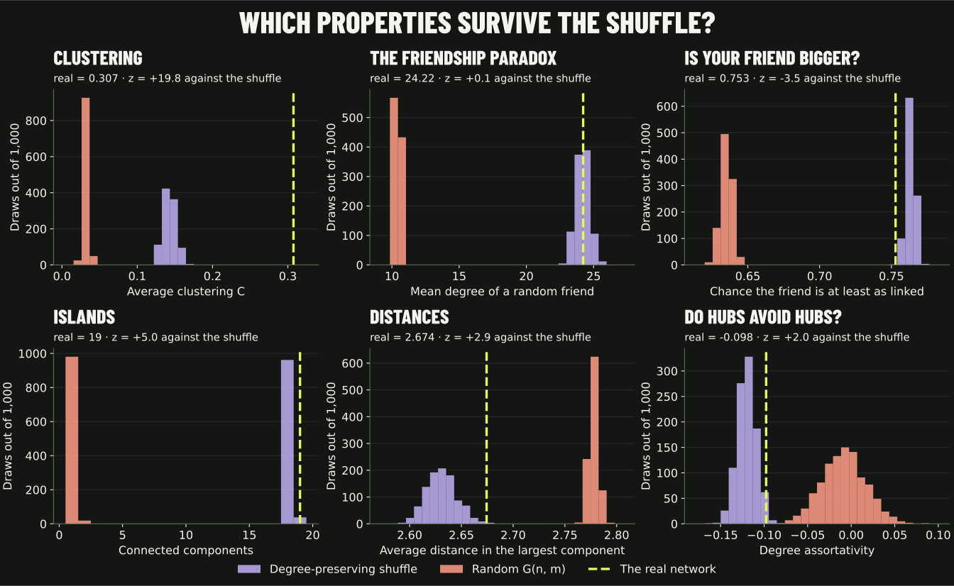
Some quantities change little under degree-preserving rewiring.Whether well-linked nodes tend to link to other well-linked nodes (above 0) or to sparsely linked ones (below 0, called disassortative). is −0.098 in the data versus a null mean of −0.120 (\htmlClass{x-z}{z} = +2.0, empirical \htmlClass{x-p-empirical}{p} = 0.024). The observed network is slightly less disassortative than this baseline. The result is exploratory: these one-sided p-values are unadjusted across twelve quantities.
Mean distance is 2.674 in the largest observed component versus 2.631 under the shuffle (\htmlClass{x-z}{z} = +2.9, empirical \htmlClass{x-p-empirical}{p} = 0.005). The difference is small but not zero. Short paths alone do not establish unusual wiring; the choice of baseline matters.
Part of that gap is the shuffle merging islands into the The largest component: the biggest group of nodes that can all reach each other through links.. Swaps cannot link the 17 isolates, since a degree-zero article stays degree zero, which leaves 286 linked articles (303 minus 17). In all 1,000 draws those 286 land in a single component: the nine-character Morituri island is absorbed every time. In 962 draws the giant is exactly those 286 nodes; in the other 38, an unrelated two-article pair happens to split off elsewhere, leaving a giant of 284. A like-for-like check that holds the population fixed instead, shuffling only the 277-article core used in Screen Test, gives 2.674 against a null mean of 2.601 (\htmlClass{x-z}{z} = +5.2, from 400 shuffles at 10 swaps per link, fewer than the 1,000 draws at 20 swaps per link used elsewhere on this page).
Clustering is 0.307 versus a shuffle mean of 0.143 (sd 0.008); no draw reached the observed value. The network has 1,839 triangles versus 1,158 on average under the shuffle. Links among characters from the same teams or eras are one possible explanation, not a mechanism established by this test.
The same number, two nulls, two conclusions
Clustering is about ten times the \htmlClass{x-gnm}{G(\htmlClass{x-n-nodes}{n}, \htmlClass{x-m-links}{m})} mean (0.032), but about 2.2 times the degree-preserving mean (0.143). Holding degrees fixed reduces the apparent excess without eliminating it. The two nulls answer different questions; \htmlClass{x-gnm}{G(\htmlClass{x-n-nodes}{n}, \htmlClass{x-m-links}{m})} does not control for hubs.
The observed 19 components compare with 18.04 under degree-preserving rewiring (\htmlClass{x-p-empirical}{p} = 0.039) and about 1.02 under \htmlClass{x-gnm}{G(\htmlClass{x-n-nodes}{n}, \htmlClass{x-m-links}{m})} (\htmlClass{x-z}{z} = +131.6). The shuffle retains the 17 isolates, and it absorbs the nine-character Morituri island into the giant component in every one of the 1,000 draws: the largest component averages 285.9 nodes versus the observed 277 (\htmlClass{x-z}{z} = −23.3). The draws that reach 19 components (38 of 1,000) do so because a different, unrelated pair of articles splits off elsewhere, not because the shuffle keeps the Morituri island separate. Treat the component-count p-value as exploratory: matching the real count of 19 does not mean the null reproduces the island structure.
Clustering, with its baseline
Average clustering is 0.307, compared with 0.143 (sd 0.008) in 1,000 degree-preserving shuffles. The observed value exceeds every draw (empirical \htmlClass{x-p-empirical}{p} = 0.001 with the add-one correction). The degree sequence explains part of the difference from \htmlClass{x-gnm}{G(\htmlClass{x-n-nodes}{n}, \htmlClass{x-m-links}{m})}, but an excess remains after controlling for degrees.
Why do your neighbours tend to have more links?
Why a random neighbour tends to have more links
THE FRIENDSHIP PARADOX · 286 LINKED ARTICLESPick a Marvel character with at least one link. On average they have 10.0 links. Now pick one of their friends at random: that friend has 24.2. Three times out of four (75.3%) the friend is at least as linked as the character you started from. Nobody is lying; picking a friend is Picking in a way that favours nodes with more links: following a link lands on a hub far more often than picking a node at random does., because a hub is a friend to many and therefore keeps getting picked.
For a uniformly selected linked article followed by one random neighbour, the observed mean is 24.22 versus a shuffle mean of 24.19 (\htmlClass{x-z}{z} = +0.1, \htmlClass{x-p-empirical}{p} = 0.47). This quantity can change with rewiring. The edge-sampled mean, \htmlClass{x-edge-degree}{\htmlClass{x-k2-avg}{\langle k^2 \rangle} / \htmlClass{x-k-avg}{\langle k \rangle}} = 22.08, is different: it depends only on degrees and is exactly preserved.
The paradox itself follows from the degree sequence alone: scrambling who links to whom leaves the average friend's degree at 24.19, almost exactly the observed 24.22. Its per-character form tells a different story. The share of linked articles whose random friend is at least as linked as they are is 75.3% in the real network against a shuffle mean of 76.3% (\htmlClass{x-z}{z} = −3.5) — below every one of the 1,000 draws. By this measure Marvel is slightly less paradoxical than degree-preserving rewiring predicts.
It does not need hubs to exist, only variance. Under random \htmlClass{x-gnm}{G(\htmlClass{x-n-nodes}{n}, \htmlClass{x-m-links}{m})}, where the biggest article has around 19 links, the paradox weakens but refuses to die: 10.44 for a random friend against 9.47 for a random character. A The spread of link counts a fully random network gives: most nodes near the average, few far from it. still has a variance, and a variance is all the paradox asks for.
The two characters nobody out-links
The paradox has an edge case worth chasing: is there anyone whose friends are never better connected than they are? Across all 286 linked articles, exactly two.
Spider-Man is the largest hub, with 106 links. Radian has six links on the nine-character Morituri island, where no neighbour has more. Both are Nodes with at least as many links as every one of their neighbours., despite their very different degrees.
The shuffle produces 1.26 local maxima on average versus the observed two (\htmlClass{x-z}{z} = +1.3, \htmlClass{x-p-empirical}{p} = 0.205). \htmlClass{x-gnm}{G(\htmlClass{x-n-nodes}{n}, \htmlClass{x-m-links}{m})} gives 16.7 on average. These comparisons do not establish that the observed pair is exceptional.
Which articles were already separate?
MARVEL TRANSIT AUTHORITY / SERVICE BOARD
Explore the 16-station interchange map
The interchange map
16 HUBS · SCHEMATIC · UNDIRECTEDThis is a readable overview of the 16 best-connected articles (four tie at 27 links for the last two places; we keep the first two alphabetically, Emma Frost and Hank Pym). Select a line to follow its actual links. The full journey planner below includes every article.
Positions are not geography. Line colours are drawing aids, not detected communities. The map intentionally omits smaller stations; no full-network conclusion is inferred from this overview.
Plan a route through all 303 articles
Where would you like to go?
FULL 303-ARTICLE PLANNERThe planner respects the active closure after its result is revealed. Restore service to compare. It uses breadth-first search; every hop is a real link in the selected graph.
What can this dataset tell us?
What the data means
303 article entries and 1,784 directed links from the course’s frozen 26 August 2026 snapshot. A link means one article links to another within this roster. It does not measure friendship, hero strength, popularity or the whole Marvel universe.
Download the snapshot and metrics (JSON)Limits of the experiment
Only within-roster links are observed. Closing a station means deleting an article node, not predicting a real outage. The route drawn is one shortest path, not necessarily the only one. The benchmark holds degrees fixed but changes other structure.
Technical methods & code
Closures operate on the simple undirected 277-node, 1,421-edge main component. After one closure, 276 nodes remain. All four displayed results are recomputed in-browser. The recorded benchmark has 1,000 connected degree-preserving rewires per tested article; each accepts 20 swaps per edge, with a separate 50-swaps-per-edge sensitivity run. The 16-hub drawing uses an A way to split the links into lines: take a long route, remove its links, and repeat, so each link belongs to one line.. Route finding includes all 303 nodes and explicitly selects directed or undirected travel.
The twelve-quantity shuffle test is a separate run on a wider graph: the whole 303-article snapshot as simple undirected links, and deliberately not conditioned on connectedness, which is what lets the number of islands vary under the null. 1,000 draws per null, 20 successful swaps per link for the degree-preserving one and gnm_random_graph(303, 1434) for the random one. Every shuffle draw asserts that the degree sequence is unchanged before it is measured. Empirical tails are (\htmlClass{x-tail-plus-one}{1} + \htmlClass{x-extreme}{\text{draws at least as extreme}}) / (\htmlClass{x-tail-plus-one}{1} + \htmlClass{x-n-draws}{\text{draws}}), one-sided and unadjusted across the twelve quantities, so treat any single p near 0.05 as a hint rather than a result. A finite swap chain approximates the null ensemble rather than sampling it uniformly.
The random null matches the course's random Marvel network. Across the 1,000 random draws the biggest hub has 19 links on average and the average distance is 2.78; the course brief gives about 19 and 2.8, drawing each link with \htmlClass{x-p-link}{p} = 0.031 where we fix the number of links. See analysis/course_reference.py.
Analysis and source code on GitHub. All experiments run locally in your browser; the frozen data is never edited.
AI use and authorship
Built with AI assistance for interface design, programming, explanation drafts and test construction. Metrics come from the provided snapshot and reproducible analysis; the games and metaphors are authored presentation choices. Numerical checks compare independent Python and browser implementations.